MI Preprint Series
Mathematics for Industry
Kyushu University
Effect of Compressibility on
Heat-loss and Darrieus-Landau
Instability of a Premixed Flame
Keigo Wada
& Yasuhide Fukumoto
MI 2018-2
( Received April 9, 2018 )
Institute of Mathematics for Industry
Graduate School of Mathematics
Effect of Compressibility on Heat-loss and Darrieus-Landau Instability of
a Premixed Flame
Keigo Wada
1∗and Yasuhide Fukumoto
2†1Graduate School of Mathematics, Kyushu University, 744 Motooka, Nishi-ku, Fukuoka 819-0395, Japan
2Institute of Mathematics for Industry, Kyushu University, 744 Motooka, Nishi-ku, Fukuoka 819-0395, Japan
Abstract
The effect of compressibility on the stability of a premixed flame front is studied theoretically in the form ofM2 expansions
for small Mach numbers. The method of matched asymptotic expansions are used to derive jump conditions for hydrodynamic variables across a flame front which is separated into the preheat zone and the reaction zone sandwiched in the former. Our analysis captures the heat-loss caused by pressure variation in the heat-conduction equation, a manifestation of the compress-ibility effect. For calculating the dispersion relation for waves on a planar flame front, we impose translational symmetry to the temperature and the density perturbations in order to obtain the mass-flux condition at the front. We show that, if the Prandtl number and the heat release are sufficiently large, the compressibility effect suppresses the Darrieus-Landau instability.
1
Introduction
A premixed flame front is very thin (∼ 10−4 m) in
the hydrodynamic scale and can be viewed as a density discontinuity surface with a series of complicated chem-ical reactions occuring in it [1]. Darrieus [2] and Landau [3, 4] independently addressed the linear stability of a planar flame front to disturbances making wavy defor-mations and concluded that the front is unstable for any wave number. This is called the Darrieus-Landau instability (DLI). It should be born in mind that the DLI analysis prescribes a constant flame speed. In the laboratory experiment, rather than instability, a stable flame front is observed. In order to improve the DLI, Markstein [5] proposed the effect of the curvature on the flame speed phenomenologically and obtained a stable flame front for short enough wavelengths. Eckhaus [6] found that the flame speed is affected, in addition to the curvature effect, by more factors such as the rate of change of the tangential velocity and the diffusion prop-erties of the mixture. Since then, many attempts are made at deriving the jump conditions for hydrodynamic variables across the flame front [7, 8, 9, 10, 11, 12].
The flame speed condition was explored by using the matched asymptotic expansions whereby its dependence on stretching of the flame front was revealed [8, 9].
Un-∗[email protected] †[email protected]
der a common assumption of large activation energy, a coupled system of the heat-conduction and the diffu-sion equations, endowed with a chemical reaction term, are integrated in the reaction zone which constitutes the core of the flame front. In addition, the other jump conditions of the velocity and the pressure across the re-action layer were also obtained [7, 10]. These conditions are used to study the diffusive or conductive instability in order to understand the behavior of the cellular and oscillatory flame front [13].
Another asymptotic expansion is based on the relative thickness of the preheat zone to the hydrodynamic zone and leads us to jump conditions for physical quantities across a flame front, including the DL’s assumption sup-plemented by correction terms [11, 14]. In most cases, the flow field is assumed to be incompressible, with zero Mach number condition, and the pressure change is left out in the heat-conduction equation. As a consequence, in the linear analysis, perturbations of the density and the temperature do not appear and the problem focuses on purely hydrodynamic modes like DL’s.
[15, 16]. For a free space, the compressibility effect on the DLI is yet to be examined. In this investigation, the dispersion relation for waves on a compressible planar flame front is sought. Kadowaki [17, 18] employed the same assumption as the original DLI [2, 3, 4] and con-cluded that the compressibility enhances the DLI. By-chkov et al. [19] derived the mass-flux condition with allowance for the density perturbation in contrast to DLI, though restricted to perturbations complying with the translational symmetry. In case the viscous effect is ignored, the compressibility increases the perturbation growth rate [24]. Here, we take account of the viscous effect as well.
We consider the compressibility effect in the form of theM2
expansions for small Mach numbers (Ma ≪1) as exposed in Sec. 2. The leading-order terms inM2
a corre-spond to the incompressible case and the nextM2
a terms are new, which reflects the compressibility effect. This method enables us to incorporate the pressure change into the heat-conduction equation resulting in the tem-perature jump across the reaction layer. Our analysis successfully capture the temperature decrease at the exit of the reaction layer which is attributed to the heat-loss effect [1, 20, 21]. In addition, the compressibility effect has the character of increasing the maximum temper-ature higher than the adiabatic one. In deriving the jump conditions at the flame surface across the reaction layer and then preheat layer to O(M2
a), the matched asymptotic expansions with respect to two-scale factors are developed in Secs. 3 and 4. In this paper, we do not elaborate the reaction term, but instead, resort to the translational symmetry to get the mass-flux condition at the flame surface. As described in Sec. 5, the re-sulting mass-flux is zero to leading order in the relative thickness of the reaction to the preheat layers. At first order, the effect of the curvature and the viscosity come into play. In Sec. 6, the dispersion relation of a pla-nar flame front is calculated, showing that the DLI can be stabilized by the compressibility depending on the Prandtl numberP r (=kinematic viscosity/thermal dif-fusivity) and the heat releaseq. We shall show that the compressibility suppresses the DLI forP r and qlarger than certain values. Sec. 7 is devoted to a summary and preliminary result for a general case without employing the translational symmetry. Appendix A derives the mass flux at the flame front toO(δM2
a), and Appendix
B writes out the solutions for perturbation.
2
Governing Equations
We deal with the following dimensionless governing equations [11, 21]:
∂R
∂t +∇ ·(RV) = 0, (1)
R
(∂V
∂t + (V· ∇)V
)
= − 1
γM a2∇P (2)
+δP r
(
∆V+1
3∇(∇ ·V)
)
,
R
(
∂T
∂t + (V· ∇)T
)
=δ∆T+qQ (3)
+γ−1
γ
(∂
∂t +V· ∇
)
P,
R
(∂Y
∂t + (V· ∇)Y
)
= δ
Le∆Y −Q , (4)
P=RT . (5)
Here the nondimensional variables, R, V = (U, V, W),
T, P and Y are respectively the density of the mix-ture, the velocity field, the temperamix-ture, the pressure and the mass fraction of deficient species which is con-sumed through the chemical reaction. All of the vari-ables are made dimensionless with use of the valuvari-ables of the fresh mixture at a position far from the flame front, denoted by R−∞,W−∞,T−∞,P−∞ and Y−∞. The
pa-rameterld =λ/R−∞cpW−∞, withλbeing the thermal
conductivity and cp being the specific heat at constant pressure of the mixture, is used for the scale factor of the preheat zone.
δ=ld
L (6)
is its thickness relative to the hydrodynamic length scale
L. The Mach number is defined by Ma = W−∞/cs where cs = (γP−∞/R−∞)1/2 is the adiabatic sound
speed defined in the fresh mixture, with γ being the ratio of the specific heats. The Lewis number is defined byLe=λ/R−∞Dcp, with D being the diffusion
coeffi-cient of the deficoeffi-cient species, and the Prandtl number is defined byP r =µcp/λ, withµ being the coefficient of viscosity.
In the heat-conduction equation (3),qis the heat re-lease. We adopt an overall one-step irreversible chemical reaction and the reaction order is taken to be unity. The mass production rateQis assumed to be the Arrhenius type:
Q=ΛRY
δϵ2 exp
(T
b
ϵ
T−Tf
T
)
. (7)
Here, Λ andTbare the prefactor and the adiabatic tem-perature which is the value for a incompressible steady planar flow. Tf is the flame temperature which is eval-uated at the edge of the reaction sheet in the burned side. With use of nondimensional activation energyN, the scale factor of the reaction zone is provided by
ϵ=T
2
b
N . (8)
In the limit of large activation energy,N ≫1,ϵ is the small parameter.
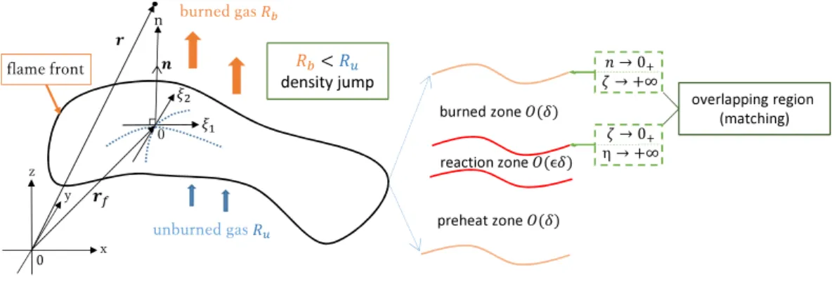
Furthermore, we introduce the curvilinear coordinate system (ξ1, ξ2, n) attached to a flame front to deduce the
jump conditions across it, by using the matched asymp-totic expansions [22].
r=rf+nn, (9)
whererf(ξ1, ξ2, t) is the position of a flame front at time
t, parametrised byξ1 andξ2, andn(ξ1, ξ2, t) is the unit
normal vector to the front which points in the direction of the burned gas. Then the normal velocity of the flame front is defined by
Wf =−∂n
∂t.
Here,Wfis chosen in such a way that a flame front prop-agates towards the unburned mixture. The time rate of change of an arclength along the coordinate curves ξ1
andξ2 are expressed by
(Uf, Vf) =
(∂ξ
1
∂t , ∂ξ2
∂t
)
.
We put
Vf = (Uf, Vf, Wf).
The flame speed Sf represents the longitudinal flame front velocity relative to the longitudinal velocity of the fluid.
Sf =W−Wf. (10)
It is convenient to introduce the mass fluxM:
M =RSf. (11)
With a view to taking compressibility into account, we expand all the functions in powers of a small parameter
M2
a as
R=R0M +Ma2R2M, P = 1 +γMa2P2M+γMa4P4M,
V=V0M+Ma2V2M,Vf =Vf0M +Ma2Vf2M,
T =T0M +Ma2T2M, Tf =Tb+Ma2Tf2M, (12)
Y =Y0M +Ma2Y2M, M=M0M +Ma2M2M,
Λ = Λ0M +Ma2Λ2M.
TheO(M2
a) term of the flame temperature can be dev-ided into the adiabatic and the non-steady parts.
Tf2M =T2M(ξ1, ξ2,0+, t) =Tb2M +T2′M(ξ1, ξ2,0+, t).
Non-steady part is important for studying the reaction term to O(M2
a). In this paper, we do not treat the details but handle only the adiabatic temperature. The detailed description is left for the next work.
3
Reaction Zone
The analysis of the reaction zone is made as an ex-tension of those of Matkowsky and Sivashinsky [7, 10]. We seek large activation energy asymptotics, under the assumption ofϵ≪1. The previous results are recovered to the leading term inM2
a. We proceed to the next order in order to gain the compressibility effect. This effect is made clear by the temperature distribution which is characterized by the heat loss and the variation of the maximum temperature.
We introduce the inner variable η for the coordinate normal to the front in the reaction zone, by the stretch-ing transformation n = ϵη. The Lewis number is as-sumed to be close to unityLe= 1 +ϵl withO(1) con-stantl. The terms ofO(M2
a) are expanded in powers of
ϵas follows: In the outer region atO(M0
a),
R0M = ˆR0+ϵRˆ1, T0M = ˆT0+ϵTˆ1,
V0M = ˆV0+ϵVˆ1, Y2M = ˆY0+ϵYˆ1, (13)
M0M = ˆM0+ϵMˆ1,
and atO(M2
a),
Ͳ
] \
[
Q
EXUQHGJDV
XQEXUQHGJDV௨ IODPHIURQW
࢘
ଶ
ଵ
ܴ൏ܴ௨ ĚĞŶƐŝƚLJũƵŵƉ
ƌĞĂĐƚŝŽŶnjŽŶĞሺϵሻ
ďƵƌŶĞĚnjŽŶĞሺሻ ŽǀĞƌůĂƉƉŝŶŐƌĞŐŝŽŶ;ŵĂƚĐŚŝŶŐͿ
՜ Ͳା Ʉ ՜ λ
՜ Ͳା
՜ λ
ƉƌĞŚĞĂƚnjŽŶĞሺሻ
Fig 1: Coordinate system attached to flame front and its inner structure. Matching is performed in overlapping region.
V2M = ˆV2M,0+ϵVˆ2M,1, Y2M = ˆY2M,0+ϵYˆ2M,1, (14)
P2M = ˆP2M,0+ϵPˆ2M,1, P4M = ˆP4M,0+ϵPˆ4M,1,
M2M = ˆM2M,0+ϵMˆ2M,1.
For O(M0
a), P0M = 1 and has been left out. In the reaction region atO(M0
a),
R0M = ˆρ0+ϵρˆ1, T0M = ˆθ0+ϵθˆ1,
V0M = ˆv0+ϵvˆ1, Y2M =ϵˆc1, (15)
and atO(M2
a),
R2M = ˆρ2M,0+ϵρˆ2M,1, T2M = ˆθ2M,0+ϵθˆ2M,1,
V2M = ˆv2M,0+ϵvˆ2M,1, Y2M = ˆc2M,0+ϵˆc2M,1, (16)
P2M = ˆp2M,0+ϵpˆ2M,1, P4M = ˆp4M,0+ϵpˆ4M,1.
M2M = ˆm2M,0+ϵmˆ2M,1.
By definition, the velocity of the flame front does not depend on the normal coordinate n, so that it has the same expansion form in both regions.
Vf0M = ˆVf0+ϵVˆf1, Vf2M = ˆVf2M,0+ϵVˆf2M,1.
The leading-order temperature ˆθ0needs to coincide with
the value of the adiabatic temperature, ˆθ0=Tb= 1 +q, a constant. To leading order inϵ, the governing equa-tions in the reaction zone are written as follows: At
O(M0
a),
(
∂ ∂t+Uf0
∂ ∂ξ1
+Vf0
∂ ∂ξ2
)
ˆ
ρ0+
∂mˆ1
∂η (17)
+ 1
a1a2
{ ∂
∂ξ1
(a2ρˆ0uˆ0) +
∂ ∂ξ2
(a1ρˆ0vˆ0)
}
−κρˆ0wˆ0= 0,
∂2vˆ 0
∂η2 =0, (18)
∂2wˆ 0
∂η2 = 0, (19)
−∂pˆ2M,0
∂η +
4 3δP r
∂2wˆ 1
∂η2 = 0, (20)
1 = ˆρ0θˆ0, 0 = ˆρ1θˆ0+ ˆρ0θˆ1 . (21)
Here,a1anda2are the scale factors ofξ1- andξ2-curve
respectively and κ is twice the mean curvature. The last equation (21) found in ref [10], and (17)-(20) were analyzed by the previous work [22]. AtO(M2
a),
∂mˆ2M,0
∂η = 0, (22)
∂2vˆ 2M,0
∂η2 =0, (23)
δ2∂ 2θˆ
2M,0
∂η2 +qQˆ2M,0= 0, (24)
δ2∂ 2cˆ
2M,0
∂η2 −Qˆ2M,0= 0, (25)
γpˆ2M,0= ˆρ2M,0θˆ0+ ˆρ0θˆ2M,0 . (26)
The matching conditions in the overlapping region be-tween the reaction zone and the outer (preheat) zone reads, for example, for the normal velocity,
ˆ
w0η→±∞= ˆWn→0±, (27)
ˆ
w1±∞= ˆW1±+η
∂Wˆ0
∂η ±
, (28)
∂wˆ0
∂η ±∞
= 0, (29)
∂wˆ1
∂η ±∞
= ∂Wˆ0
∂η ±
. (30)
The same is true for the other quantities.
Integrating (22), we find ˆm2M,0(ξ1, ξ2, t), an arbitrary
Fig 2: Temperature distribution in the reaction zone for a steady planar flow withϵ= 0.01, q= 6, γ = 1.4,
P r= 1. ˆθ1= 0 corresponds to the edge of the reaction
zone in the burned side.
gives
[ ˆM2M,0] = 0, (31)
where [ ˆM2M,0] = ˆM2M,0(n = 0+)−Mˆ2M,0(n = 0−)
denotes the jump across the reaction sheet. Next, integrating (23), we get
∂vˆ2M,0
∂η =A(ξ1, ξ2, t), (32)
where A is an arbitrary function of ξ1, ξ2 and t. Due
to (29), the integral constant A is found to be zero. As a consequence, we know that the velocity field is continuous across the reaction layer.
[
ˆ V2M,0
]
= 0. (33)
Similarly, combining (24) and (25) so as to eliminate the reaction term, the jump condition for the enthalpy is obtained as
[
ˆ
T2M,0+qYˆ2M,0
]
= 0. (34)
Finally, in order to get the temperature jump across the reaction layer, we use theO(M0
a) equations (17), (18), (19) and (21) showing that
∂mˆ1
∂η (ξ1, ξ2, t), (35)
an arbitrary function of ξ1, ξ2 and t, because ˆρ0 and
the velocity field (ˆu0,ˆv0,wˆ0) are independent ofη. On
the other hand, from the definition of the mass flux (11) with (21), we find that
∂wˆ1
∂η = ˆm0 ∂θˆ1
∂η + ˆθ0 ∂mˆ1
∂η . (36)
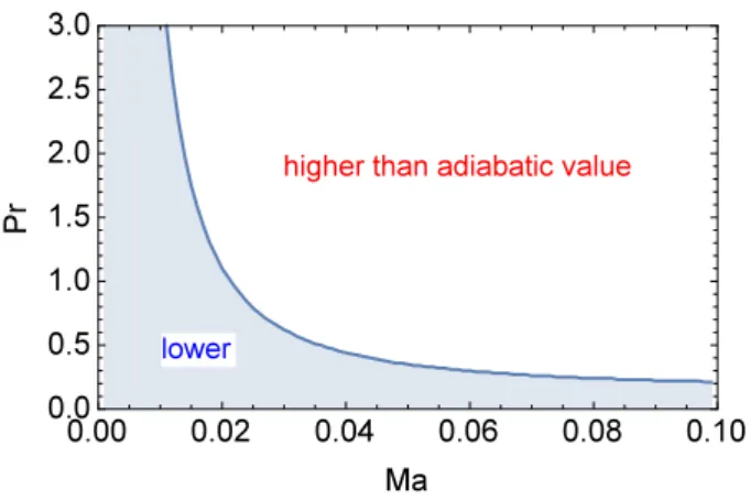
Fig 3: Boundary of maximum of temperature in the reaction zone for a steady planar flow with ϵ = 0.01,
q= 6, γ= 1.4.
We recall, from the definition, the temperature has the following form in the reaction zone.
T = 1 +q+ϵθˆ1+Ma2θˆ2M,0 . (37)
In the incompressible case [10], the temperature gradi-ent of O(ϵ0
M0
a) is assumed to be zero at the reaction layer in the burned side,
∂θˆ1
∂η+∞
= ∂Tˆ0
∂n+= 0. (38)
From this assumption, where the temperature gradient ofO(ϵ0
M0
a) has a finite value in the unburned side, we see that ˆθ1 varies from −∞ to ˆT1+ monotonically and
the position where ˆθ1 = ˆT1+ towards the edge of the
reaction zone. Based on (38), the temperature gradient ofO(ϵ1M0
a) can be expressed in the reaction zone as
∂θˆ1
∂η = q δ
(
eTˆ1+−(1 + ˆT
1+−θˆ1)e ˆ
θ1) 1 2
. (39)
Using (35),(36) and (38), we find from (20) and (26) the expression of ˆθ2M,0 to be
ˆ
θ2M,0=
4
3δP rγθˆ0mˆ0
∂θˆ1
∂η + ˆT2M,0+, (40)
Eventually we get from equation (40) the temperature jump condition
[
ˆ
T2M,0
]
=−4
3δP rγ
(
ˆ
M0
ˆ
R0
∂Tˆ0
∂n
)
−
. (41)
should emphasize that the heat loss and the maximum temperature variation are brought by the compressibil-ity effect. Equation (40) implies that, unlike the incom-pressible case, the peak of the temperature does not sit at the edge but moves into the reaction zone. Fig-ure 2 shows the temperatFig-ure profile for a steady pla-nar flow. In addition to the increase of the maximum temperature with Ma, the temperature at the exit of the reaction layer rapidly decreases, which results in the heat loss influenced by the compressibility. This is at-tributed to the pressure variation in the heat-conduction equation which is equivalent to the volumetric heat-loss term [1, 20, 21]. There is also a possibility for the peak temperature to overshoot the adiabatic temper-ature ˆθ0= 1 +q, the value for the incompressible case.
This depends on the Prandtl numberP r and the Mach numberMa. This relation is displayed in Fig. 3. IfP r
is small enough, the peak temperature is lower than the adiabatic temperature. However, the compressibility ef-fect is capable of raising the peak temperature beyond the adiabatic one forP rlarger than a certain value.
4
Preheat Zone
Now we take the limit of δ ≪ 1, under the condi-tion ϵ ≪ δ so that the reaction layer is embraced in the preheat zone. We introduce the stretched coordi-nate n =δζ where ζ is the inner variable for the pre-heat zone. The leading-order terms in M2
a are analo-gous to the ones obtained by the analysis of Matalon and Matkowsky [11]. Our task is to go beyond to the next order in M2
a, and, to this aim, all the dependent variables are expanded in powers ofδ.
In the hydrodynamic zone, we write
ˆ
R2M,0=R2M,0+δR2M,1, Tˆ2M,0=T2M,0+δT2M,1,
ˆ
V2M,0=V2M,0+δV2M,1,Yˆ2M,0=Y2M,0+δY2M,1,
ˆ
P2M,0=P2M,0+δP2M,1, Pˆ4M,0=P4M,0+δP4M,1.
ˆ
M2M,0=M2M,0+ϵM2M,1.
In the preheat zone, we write
ˆ
R2M,0=ρ2M,0+δρ2M,1, Tˆ2M,0=θ2M,0+δθ2M,1,
ˆ
V2M,0=v2M,0+δv2M,1, Yˆ2M,0=c2M,0+δc2M,1,
ˆ
P2M,0=p2M,0+δp2M,1, Pˆ4M,0=p4M,0+δp4M,1.
ˆ
M2M,0=m2M,0+ϵm2M,1.
To leading order inδ, the governing equations in the preheat zone are reduced to
∂m2M,0
∂ζ = 0, (42)
m2M,0
∂v⊥0
∂ζ + ∂2v
⊥2M,0
∂ζ2 =P r
∂2v
⊥2M,0
∂ζ2 , (43)
m2M,0
∂w0
∂ζ + ∂2w
2M,0
∂ζ2 =−
∂p4M,0
∂ζ +
4 3P r
∂2w 2M,0
∂ζ2 ,
(44)
m2M,0
∂c0
∂ζ + ∂c2M,0
∂ζ = ∂2c
2M,0
∂ζ2 −Q2M,0, (45)
m2M,0
∂θ0
∂ζ + ∂θ2M,0
∂ζ = ∂2θ
2M,0
∂ζ2 +qQ2M,0
+(γ−1)(w0−wf0)
∂p2M,0
∂ζ . (46)
Here,v⊥0, w0, θ0, p2M,0have been obtained atO(Ma0).
θ0=
{
T0−+ em0ζ (ζ <0),
T0+ (ζ >0). (47)
w0=
{
m0θ0+wf0 (ζ <0),
W0+ (ζ >0).
v⊥0=v⊥0(ξ1, ξ2, t).
p2M,0=
P2M,0−+
(4
3P r−1
)
m2
0[[T0]]em0ζ (ζ <0),
P2M,0+ (ζ >0).
Here, [[T0]] = T0(n = 0+)−T0(n = 0−) denotes the
jump across the flame front in the hydrodynamic zone. In an analogous way with the reaction zone, integrat-ing the equations (42),(43),(44),(45) and (46) with the matching conditions (31),(33),(34) and (41), we manip-ulate the following jump conditions
[[m2M,0]] = 0, (48)
[[v⊥2M,0]] =0, (49)
[[P4M,0]] =−m0[[W2M,0]]−m2M,0[[W0]], (50)
[[θ2M,0]] +q[[c2M,0]]
= (γ−1)m2 0[[T0]]
{
−4
3P rT0++
(
4 3P r−1
) (
T0−+
[[T0]]
2
)}
.
(51)
5
Translational Symmetry
ܨሺݔǡݕǡݐሻ
ݖ
ƉůĂŶĂƌĨƌŽŶƚ ;džͲLJƉůĂŶĞͿ
ƉĞƌƚƵƌďĞĚĨƌŽŶƚ
ܶത ݖ ƐƚĞĂĚLJƉůĂŶĂƌ ܶത ݖܨ ܶᇱሺݔǡݕǡݖܨǡݐሻ
ƉĞƌƚƵƌďĞĚ
ĞƋƵŝǀĂůĞŶƚ͗ƚƌĂŶƐůĂƚŝŽŶĂůƐLJŵŵĞƚƌLJ
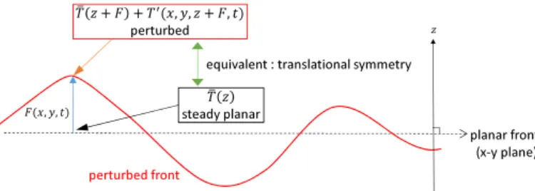
Fig 4: Translational symmetry.
The subsequent investigations [5, 11] made an effort to derive it by looking into the energy and the mass frac-tion equafrac-tions in the reacfrac-tion zone. The energy and the heat-conduction equations are not easy to handle in the reaction zone. By leaving the detailed analysis to our next paper, we seek, in this investigation, a restricted solution constrained by translational symmetry [19].
5.1
Equations for perturbations with
symmetry
The perturbed heat-conduction equation, valid in the preheat zone, is derived from (3).
¯ R∂T ′ ∂t + ¯ M δ ∂T′ ∂ζ + M′ δ dT¯
dζ =δ ( 1 δ2 ∂2
∂ζ2+ ∆⊥
)
T′
+γ−1
γ
(∂P′
∂t + ¯ W δ ∂P′ ∂ζ + W′ δ dP¯
dζ
)
. (52)
Here, the terms with overbar and a prime mean the steady planar and the perturbed functions respectively. The mass flux of the flow has the following form.
M =RW. (53)
We focus on the perturbations of the temperature and the density that have the translational symmetry at the flame front in the hydrodynamic zone. The calculation is performed on the unburned side of the preheat zone in such a way that the gradient of the temperature exists in the overlapping region with the hydrodynamic one.
The assumption of translational symmetry is dictated by
T′
=−FdT¯ dz =−
F δ
dT¯ dζ, R
′
=−FdR¯ dz =−
F δ
dR¯ dζ,
(54)
whereF(x, y, t) is a small-amplitude displacement of the perturbed flame front (Fig.4). Then, from (5), the pres-sure also has the same symmetry.
P′
=R′¯
T+ ¯RT′
=−FdR¯
dzT¯−RF¯ dT¯
dz =−F dP¯
dz. (55)
In the regime M2
a ≪ 1, M2 expansions are given as follows.
¯
T = ¯T0M +Ma2T¯2M, R¯= ¯R0M +Ma2R¯2M, ¯
W = ¯W0M +Ma2W¯2M, M¯ = ¯M0M+Ma2M¯2M, ¯
P = 1 +γM2
aP¯2M +γMa4P¯4M,
T′
=T′
0M +M
2
aT
′
2M, R
′
=R′
0M +M
2
aR
′
2M,
W′
=W′
0M +M
2
aW
′
2M, M
′
=M′
0M+M
2
aM
′
2M,
P′
=γM2
aP
′
2M +γM
4
aP
′
4M, F=F0M+Ma2F2M. (56)
With (56), the perturbations (54) and (55) are expanded inM2
a as
T′
0M =−
F0M
δ dT¯0M
dζ , T
′
2M =−
F2M
δ dT¯0M
dζ − F0M
δ dT¯2M
dζ ,
R′0M =−
F0M
δ dR¯0M
dζ , R
′
2M =−
F2M
δ
dR¯0M
dζ − F0M
δ
dR¯2M
dζ ,
P′
2M =−
F0M
δ dP¯2M
dζ , P
′
4M =−
F2M
δ dP¯2M
dζ − F0M
δ dP¯4M
dζ .
(57)
Subsequently, we shall gain the perturbed mass flux (75) and (79) on the unburned side of the flame front, by Substituting these into (52).
Under the conditions ofϵ≪1 andδ≪1, asymptotic expansions of the steady planar solution and the small amplitude perturbations in the preheat zone are given, up toO(δ2), by
¯
T0M = ¯θ0+δθ¯1+δ2θ¯2, T¯2M = ¯θ2M,0+δθ¯2M,1+δ2θ¯2M,2,
¯
R0M = ¯ρ0+δρ¯1+δ2ρ¯2, R¯2M = ¯ρ2M,0+δρ¯2M,1+δ2ρ¯2M,2,
¯
W0M = ¯w0+δw¯1+δ2w¯2, W¯2M = ¯w2M,0+δw¯2M,1+δ2w¯2M,2,
¯
M0M = ¯m0+δm¯1+δ 2
¯
m2,M¯2M = ¯m2M,0+δm¯2M,1+δ 2
¯
m2M,2,
F0M =F0+δF1+δ 2
F2, F2M =F2M,0+δF2M,1+δ 2
F2M,2,
1 = ¯p0+δp¯1 +δ 2
¯
p2,
¯
P2M = ¯p2M,0+δp¯2M,1+ δ 2
¯
p2M,2,
¯
P4M = ¯p4M,0+δp¯4M,1+ δ2p¯4M,2. (58)
Using the asymptotic expansions (58), we can rewrite the perturbations (57) as
T0′M =
θ−1
δ +θ0+δθ1+δ
2
R′0M =
ρ−1
δ +ρ0+δρ1+δ
2
ρ2,
W0′M =w0+δw1+δ2w2,
T2′M =
θ2M,−1
δ +θ2M,0+δθ2M,1+δ
2
θ2M,2, (59)
R′2M =
ρ2M,−1
δ +ρ2M,0+δρ2M,1+δ
2
ρ2M,2,
W′
2M =w2M,0+δw2M,1+δ 2
w2M,2,
P2′M =
p2M,−1
δ +p2M,0+δp2M,1+δ
2
p2M,2,
P′
4M =
p4M,−1
δ +p4M,0+δp4M,1+δ
2
p4M,2,
in which each term is written, for instance, as
θ−1=−F0
dθ¯0
dζ , θ0=−
(
F1
dθ¯0
dζ +F0 dθ¯1
dζ
)
,
θ1=−
(
F2
dθ¯0
dζ +F1 dθ¯1
dζ +F0 dθ¯2
dζ
)
, . . .etc.. (60)
For the perturbation of the mass flux (53), we have, upon substitution from (56) and (59),
M′
0M =
m−1
δ +m0+δm1+δ
2
m2,
M′
2M =
m2M,−1
δ +m2M,0+δm2M,1+δ
2
m2M,2, (61)
where
m−1=ρ−1w¯0=−F0
dρ¯0
dζ w¯0,
m0=ρ0w¯0+ρ−1w¯1+ ¯ρ0w0
=−
(
F1
dρ¯0
dζ +F0 dρ¯1
dζ
)
¯
w0−F0
dρ¯0
dζ w¯1+ ¯ρ0w0,
. . .etc.. (62)
5.2
Planar Steady State
The basic state is a steady planar flow. The gov-erning equations for it is derived from (1),(2),(3) and (5). Incorporating the translational symmetry allows us to skip the mass fraction equation (4), which achieve a great simplification.
¯
M = 1, (63)
dW¯ dζ =−
1
γM2
a
dP¯ dζ +
4 3P r
d2W¯
dζ2 , (64)
dT¯ dζ =
d2T¯
dζ2 +
γ−1
γ W¯ dP¯
dζ, (65)
¯
P = ¯RT .¯ (66)
It follows from (53),(63) and (66) that
¯
R0MW¯0M = 1, 1 = ¯R0MT¯0M,
¯
R2MW¯0M+ ¯R0MW¯2M = 0, 0 = ¯R2MT¯0M + ¯R0MT¯2M (67)
We combine (64),(65) and (67) into
dP¯2M
dζ =
(
4 3P r−1
)
dT¯0M
dζ . (68)
The asymptotic expansions (58) reduce (67) and (68) to
¯
ρ0w¯0= 1, 1 = ¯p0= ¯ρ0θ¯0, (69)
¯
ρ2M,0w¯0+ ¯ρ0w¯2M,0= 0, 0 = ¯ρ2M,0θ¯0+ ¯ρ0θ¯2M,0,
(70)
dp¯2M,0
dζ =
(
4 3P r−1
)
dθ¯0
dζ . (71)
5.3
Mass Flux
First, we derive the mass flux condition for the in-compressible case. Collecting the terms of O(δ−2M0
a) in (52), we get
∂θ−1
∂ζ +m−1 dθ¯0
dζ = ∂2θ
−1
∂ζ2 .
By virtue of (60) and (62), this becomes
F0w¯0
(dθ¯
0
dζ
)2
=−F0
d dζ
(d2θ¯ 0
dζ2 −
dθ¯0
dζ
)
.
The right-hand side of this equation is zero
d2θ¯ 0
dζ2 −
dθ¯0
dζ = 0. (72)
because ¯p0 = 1 from (69), implying that the last term
of (65) vanishes. Provided that the flow velocity should not be zero, we get
dθ¯0
dζ = 0. (73)
In view of (69) and (71), this condition gives
dw¯0
dζ = dρ¯0
dζ = dp¯2M,0
dζ = 0. (74)
The terms of O(δ−1
M0
a) do not bring any new infor-mation. We proceed to the next order and derive the same mass-flux condition as the one obtained by By-chkovet al. [19]. Collecting the terms ofO(δ0M0
a) in (52), we have
¯
ρ1
∂θ−1
∂t + ¯ρ0 ∂θ0
∂t + ∂θ1
∂ζ +m1 dθ¯0
dζ +m0 dθ¯1
dζ +m−1 dθ¯2
=∂
2θ 1
∂ζ2 + ∆⊥θ−1.
By substitution from (60),(62),(72), (73) and (74), we are left with
−F0
dρ¯1
dζ w¯0+ ¯ρ0
(
w0−
∂F0
∂t
)
= 0. (75)
Taking the outer limitζ→ −∞, forδ≪1, gives rise to the matching condition with the hydrodynamic zone on the unburned side.
R′
0−W¯0−+ ¯R0−
(
W′
0−−
∂F0
∂t
)
= 0. (76)
This is the desired mass-flux condition on the unburned side of a flame front in the hydrodynamic zone, aug-menting Landau’s assumption [3, 4] with the first term. This condition coincides with that of Bychkovet al. [19]. Their analysis forgets the last terms includingP in (3). We reach (75) through an elaborate analysis in the re-action and preheat zone on the ground of the complete heat-conduction equation.
The next-order solution inδ, in the preheat zone, pro-vides us with the curvature effect, embodying the Mark-stein effect [5] (Appendix A).
We are now in a position to deduce the mass flux on the unburned side of the flame front, with the com-pressibility effect taken into account, based on the heat-conduction equation. Collecting the terms ofO(δ−2
M2
a) in (52), we have
∂θ2M,−1
∂ζ +m2M,−1 dθ¯0
dζ +m−1 dθ¯2M,0
dζ
= ∂
2
θ2M,−1
∂ζ2 + (γ−1) ¯w0
∂p2M,−1
∂ζ .
By use of (73) and (74), this equation becomes
∂ ∂ζ
(
−F0
dθ¯2M,0
dζ ) = ∂ 2 ∂ζ2 (
−F0
dθ¯2M,0
dζ
)
.
This is satisfied by the heat-conduction equation (65) because of (74).
Collecting the terms ofO(δ−1
M2
a) in (52), we have
¯
ρ2M,0
∂θ−1
∂t + ¯ρ0
∂θ2M,−1
∂t + ∂θ2M,0
∂ζ +m2M,0 dθ¯0M
dζ
+m2M,−1
dθ¯1
dζ +m0 dθ¯2M,0
dζ +m−1 dθ¯2M,1
dζ
= ∂
2
θ2M,0
∂ζ2 + (γ−1)
(
∂p2M,−1
∂t + ¯w1
∂p2M,−1
∂ζ
+ ¯w0
∂p2M,0
∂ζ +w0 dp¯2M,0
dζ
)
.
By use of (60),(62),(65),(73),(74) and (75), we are left with
−F0
dρ¯2M,0
dζ w¯0 dθ¯1
dζ = 0.
The temperature gradientdθ¯1/dζshould not be zero
be-cause theθ0term in (60) should not be zero on account
of the preheat zone result (47) in Sec.4. Accordingly, we have no choice but to put the density gradient zero.
dρ¯2M,0
dζ = 0. (77)
From (70), this leads to
dw¯2M,0
dζ = 0,
dθ¯2M,0
dζ = 0, (78)
with the help of (73) and (74). Collecting the terms of O(δ0M2
a) in (52), taking ac-count of (65),(73),(74),(77) and (78), we have
{
−ρ¯2M,0
∂F0
∂t −ρ¯0 ∂F2M,0
∂t −
(
F2M,0
dρ¯1
dζ +F0 dρ¯2M,1
dζ
)
¯
w0
−F0
dρ¯1
dζ w¯2M,0+ ¯ρ2M,0w0+ ¯ρ0w2M,0
}
dθ¯1
dζ
= γ−1 ¯
ρ0
(
¯
ρ0w0−ρ¯0
∂F0
∂t −w¯0F0 dρ¯1
dζ
)
dp¯2M,1
dζ .
With the help of (75), this simplifies to
−
(
F2M,0
dρ¯1
dζ +F0 dρ¯2M,1
dζ
)
¯
w0−F0
dρ¯1
dζ w¯2M,0
+ ¯ρ2M,0
(
w0−
∂F0
∂t
)
+ ¯ρ0
(
w2M,0−
∂F2M,0
∂t
)
= 0.
(79)
Matching with hydrodynamic zone, by taking the outer limitζ→ −∞, leads to
R′
2M,0−W¯0−+R′0−W¯2M,0−
+ ¯R2M,0−
(
W0′−−
∂F0
∂t
)
+ ¯R0−
(
W2′M,0−−
∂F2M,0
∂t
)
= 0. (80)
This implies that the perturbed mass flux on the un-burned side of the flame front is absent, an extension of Landau’s assumption to the compressible case. The condition (80) was also obtained by Bychkovet al. [19] based on the incomplete heat-conduction equation. We put (80) on the firm ground. We remark that the terms with ¯R0−was derived by Kadowaki [17]. The jump
We establish that, under the assumption of the trans-lational symmetry, the perturbed mass flux is zero at the flame front even when the compressibility effect is included. The compressibility affects the mass flux at the next order inδ, at which the contributions from the curvature and the viscosity play an important role (see Appendix A).
6
Hydrodynamic Instability
We are ready to look into the effect of compressibility on the DLI. We pose a small perturbation of the plane flame front in the form
F(x, y, t) =fexp(ix·k+ Ωt),
wherex= (x, y),k= (kx, ky) is the wavenumber, with
k= (k2
x+ky2)1/2, and Ω is the growth rate of the per-turbation [23]. We explore Ω in the form
Ω = Ω0+Ma2Ω2M . (81)
Any hydrodynamic variable Φ is expressed in the form
Φ = ¯Φ(z) + Φ′
(x, y, t),
Φ′
= ˜Φ(z) exp(ix·k+ Ωt). (82)
Here, ¯Φ(z) is a steady planar solution and Φ′
(z) is a small perturbation. The coordinate system attached to the flame front is
ξ=z−F(x, y, t).
The jump conditions (48),(49),(50) and (51) are applied at the flame front, ξ = 0±. To first order in Ma2, the
linearized equations of (1)-(5) are written down as
∂R′
2M,0
∂t + ¯W0 ∂R′
2M,0
∂ξ + ¯R2M,0 ∂W′
0
∂ξ + ¯R0 ∂W′
2M,0
∂ξ
+ ¯R2M,0∇⊥V′⊥0+ ¯R0∇⊥V⊥′ 2M,0= 0, (83)
¯
R2M,0
∂W′
0
∂t + ¯R0 ∂W′
2M,0
∂t + ∂W′
2M,0
∂ξ =− ∂P′
4M,0
∂ξ ,
(84)
¯
R2M,0
∂V′ ⊥0
∂t + ¯R0 ∂V′
⊥2M,0
∂t + ∂V′
⊥2M,0
∂ξ =−∇⊥P
′
4M,0,
(85)
¯
R0
∂T′
2M,0
∂t + ∂T′
2M,0
∂ξ = (γ−1)
(∂P′
2M,0
∂t + ¯W0 ∂P′
2M,0
∂ξ ) , (86) ¯ R0 ∂Y′
2M,0
∂t + ∂Y′
2M,0
∂ξ = 0, (87)
γP′
2M,0=R
′
2M,0T¯0+ ¯R0T
′
2M,0. (88)
Here the incompressible perturbations R′
0 and T
′
0 are
zero and ∇⊥ = (∂/∂x, ∂/∂y). The pressure
perturba-tion is calculated as [3, 4]
˜
P2M,0=
{
Aekξ (ξ <0),
Be−kξ (ξ >0). (89) The arbitrary constantsAandBare determined by (76) and the continuity of the pressure in theO(M0
a) analysis as
A=B=−Ω0f
(Ω
0
k + 1
)
. (90)
The perturbations of the temperature and the mass frac-tion are found, from (86) and (87), as
˜
T2M,0=
(γ−1)Aekξ (ξ <0),
Ie−Ω0Wξ+ (γ−1)W Be−kξ (ξ >0). (91)
˜
Y2M,0=
{
0 (ξ <0),
0 (ξ >0).
The perturbation of the mass fraction disappears be-cause Y = 0 on the burned side. W = 1 +q is the incompressible normal velocity of a burned gas for a steady planar flow. in the same manner as for the DLI in the incompressible case. By employing the jump con-dition (51), we find the constantI in (91) to be
I= (γ−1)(1−W)A. (92)
The solutions of the other equations are obtained in ex-plicit form and are written out in Appendix B with the upper solution corresponding to the upstream (ξ < 0) and the lower to the downstream (ξ >0). In the solu-tions, AM, BM, CM, DM and HM are arbitrary con-stants of O(M2
a) and the other leading constants C,D andH has the relation
Ω0
WH= ikxC+ ikyD. (93)
Enforcing the jump conditions (48), (49) and (50), we obtain the dispersion relation toO(M2
a) as follows:
Ω =ω0W k+M 2
Fig 5: Growth rate of the perturbation v.s. Mach num-ber in two cases of DL’s assumption (solid) [17], and translational symmetry (dot-dashed) withP r = 0 and
W = 7.
Fig 6: Growth rate of the perturbation v.s. Mach num-ber with respect to different values of Prandtl numnum-ber withW = 7.
The first term, ω0 recovers the dispersion relation for
the DLI [3, 4].
ω0=
Ω0
kW =
−W+ (W3
+W2
−W)1/2
W+W2 . (95)
The second termω2M is the correction originating from the compressibility effect.
ω2M = Ω2M
kW
= 1
4(1 +ω0+W ω0)
{
−2 ¯R2M+W(1 +ω 2 0)
+ω0(1 +W ω0)(−3−2ω0+W2ω20)
+ω0(1 +W ω0)(1 +ω0)(K−2γ(W−1) +W−W ω0)},
(96)
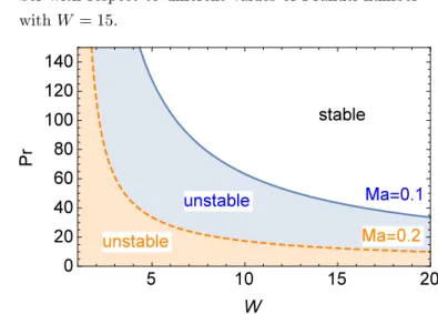
Fig 7: Growth rate of the perturbation v.s. Mach num-ber with respect to different values of Prandtl numnum-ber withW = 15.
Fig 8: Stability boundary determined by Prandtl num-ber and heat release.
in which
¯
R2M+=γ
1−W W
+ (γ−1)W−1
W2
{
1 + W−1 2
(
4 3P r+ 1
)}
,
K=
{
0 (Translational symmetry),
2(1 +γ) + 2γ(W −1) (DL’s assumption).
Here K = 0 is our case of exploiting the translational symmetry and K ̸= 0 is the case of DL’s assumption as used by Kadowaki [17]. Kadowaki considered a finite Mach number case and the resulting growth rateω2M,0
contains M2
0 and the growth rate of the perturbation is larger than that of the DLI with the increment of the Mach number as shown in Figure 5, forγ= 1.4. Figures 6 and 7 show the stabilizing effect of the compressibility on the DLI in the presence ofP r. For large values ofP r, the DLI is weakened as the Mach number Ma increases. This effect is reinforced by the heat releaseq. By comparison between Figures 6 and 7, increase inq makes deviation from the DLI larger. The dependence on P r and q is shown by Figure 8. Figure 8 reveals that large value is prefered for both parameters for the sake of stabilizing the DLI.
7
Conclusions
We have explored the effect of the compressibility by theM2 expansion on the DLI. Thanks to this method,
we can deal with a perturbation of the temperature which comes from the pressure variation in the heat con-duction equation in the compressible case. The investi-gation of the inside of the flame front, with the viscos-ity taken into account, derives the boundary conditions. From the study of the reaction layer, we have demon-strated that the temperature jump occurs in leading or-der of ϵ and push the maximum-value position of the temperature into the inside of the reaction layer. The compressibility raises the temperature at the reaction layer in the upstream (unburned side) and decreases in the downstream (burned side) as shown by Fig. 2. This decrease in the temperature at the edge corresponds to the volumetric heat-loss effect. In the previous re-searches [1, 20, 21], the sink term describing the volu-metric heat-loss effect is inserted in the heat-conduction equation artificially. However, if we employ theM2
ex-pansions method, the pressure variation terms replace the sink term naturally as a result of the compressibility effect. The increase of the temperature inside the reac-tion zone (Fig. 2) is peculiar to the compressibility effect which was not realized in the case of the additional sink term [1, 20, 21]. The values of P r and Ma determine whether the temperature (37) exceeds the adiabatic one
Tb = 1 +q or not (Fig. 3). From the analysis of the preheat zone, the jump condition (51) of the enthalpy is derived, which manifests the effect of pressure as the source term of (46).
In this investigation, we employed the assumption of the translational symmetry for the perturbation. This restricted symmetry leads to the zero mass-flux condi-tion (76) and (80) at O(δ0). At O(δ), the mass flux
is generated not only by the mean curvature effect and but also the viscosity effect, the latter being of the com-pressibility origin (Appendix A).
The dispersion relation of a planar flame front shows that large viscosity weakens the DLI, given sufficiently large heat release, even if Ma is small. We conclude that weak compressibility has a stabilizing effect on the DLI, depending on the viscosity. This conclusion has been reached by deriving the missing boundary condi-tions (76) and (80) of the mass flux, though for restricted perturbations.
In order to obtain the mass flux condition in a general case, we are requested to fully analyse the reaction zone. By performing this procedure, we find that the mass flux is nonzero even atO(δ0) owing to the compressibility.
M′
2M,0−=M ′
2M,0+=
1 2W R
′
2M,0+ .
The detailed analysis will be reported in a subsequent paper.
Acknowledgments
We are grateful to Professors Moshe Matalon and Michael Tribelsky for helpful discussions and invaluable comments. Y. F. was partially supported by a Grant-in-Aid for Scientific Research from the Japan Society of Promotion of Science (Grant No. 16K05476).
Appendix A
This appendix confirms the Markstein condition for the mass flux at O(δM0
a) [5]. Moreover, we extend the condition to the compressible case.
Collecting the terms of O(δM0
a) in (52), using (65),(73),(74) and (75), we have
−
(
F1
dρ¯1
dζ +F0 dρ¯2
dζ
)
¯
w0−F0
dρ¯1
dζ w¯1
+ ¯ρ1
(
w0−
∂F0
∂t
)
+ ¯ρ0
(
w1−
∂F1
∂t
)
+ ∆⊥F0
For the sake of attaining the fulfilment of the matching condition, one more equation is necessary, obtained by taking the derivative of (97) with respect toζ,
−
(
F1
d2ρ¯ 1
dζ2 +F0
d2ρ¯ 2
dζ2
)
¯
w0−
(
F1
dρ¯1
dζ +F0 dρ¯2
dζ
)dw¯
0
dζ
−F0
d2ρ¯ 1
dζ2 w¯1−F0
dρ¯1
dζ dw¯1
dζ + dρ¯1
dζ
(
w0−
∂F0
∂t
)
+ ¯ρ1
dw¯0
dζ + dρ¯0
dζ
(
w1−
∂F1
∂t
)
+ ¯ρ0
dw¯1
dζ = 0. (98)
Matching with the hydrodynamic zone, by taking the limitζ→ −∞of (97), leads to
−
(
F1
dR¯0
dz −+F
0
dR¯1
dz −
)
¯
W0−−F0
dR¯0
dz −
¯
W1−
+ ¯R1−
(
W0−−
∂F0
∂t
)
+ ¯R0−
(
W1−−
∂F1
∂t
)
+ ∆⊥F0
=ζ
{
F0
d2R¯ 0
dz2
−
¯
W0−+F0
dR¯0
dz −
dW¯0
dz −
−dR¯0
dz −
(
W0−−
∂F0
∂t
)
−R¯0−
dW0
dz −
}
. (99)
The right-hand side of (99) diverges in the limit ofζ→ −∞. But this difficulty is rescued by taking the outer limit (ζ→ −∞) of (98), resulting in
−F0
d2R¯ 0
dz2
−
¯
W0−−F0
dR¯0
dz −
dW¯0
dz −
+dR¯0
dz −
(
W0−−
∂F0
∂t
)
+ ¯R0−
dW¯0
dz −
= 0.
We eventually reach the mass flux ofO(δ) as the match-ing condition on the unburned side.
R′
1−W¯0−+R′0−W¯1−
+ ¯R1−
(
W′
0−−
∂F0
∂t
)
+ ¯R0−
(
W′
1−−
∂F1
∂t
)
=−∆⊥F0. (100)
This condition reveals that the mass flux is influenced by the mean curvature of the flame front, in accord with the Markstein condition [5].
Collecting the terms of O(δ1M2
a) in (52), using the conditions (65),(73),(74),(77) and (78), we have
dθ¯1
dζ
[
−ρ¯2M,1
∂F0
∂t −ρ¯2M,0 ∂F1
∂t −ρ¯1 ∂F2M,0
∂t −ρ¯0 ∂F2M,1
∂t
−
(
F2M,1
dρ¯1
dζ +F2M,0 dρ¯2
dζ +F1 dρ¯2M,1
dζ +F0 dρ¯2M,2
dζ ) ¯ w0 − (
F2M,0
dρ¯1
dζ +F0 dρ¯2M,1
dζ
)
¯
w1−
(
F1
dρ¯1
dζ +F0 dρ¯2
dζ
)
¯
w2M,0
−F0
dρ¯1
dζ w¯2M,1+ ¯ρ2M,1w0+ ¯ρ2M,0w1+ ¯ρ1w2M,0+ ¯ρ0w2M,1
]
=−∆⊥F2M,0
dθ¯1
dζ
+ (γ−1)
[(
−∂F1
∂t +F0 dw¯2
dζ +F1 dw¯1
dζ +w1
)dp¯
2M,1
dζ
+
(
−∂F0
∂t +F0 dw¯1
dζ +w0
)dp¯
2M,2
dζ
]
(101)
In order to transform the right-hand side of this equa-tion, we use (67) and (68). From (67), we know that
¯
ρ1w¯0+ ¯ρ0w¯1= 0,
¯
ρ2w¯0+ ¯ρ1w¯1+ ¯ρ0w¯2= 0.
Then, because of (74),dw¯1/dζanddw¯2/dζare rewritten
as
dw¯1
dζ =−
¯
w0
¯
ρ0
dρ¯1
dζ , dw¯2
dζ =−
¯
w0
¯
ρ0
dρ¯2
dζ − dρ¯1
dζ
¯
w1
¯
ρ0
−ρ¯1
¯
ρ0
dw¯1
dζ . (102)
From (68), we get
dp¯2M,1
dζ =
(4
3P r−1
)dθ¯
1
dζ . (103)
By use of (102),(103) and (97), we transform (101) into
−ρ¯2M,1
∂F0
∂t −ρ¯2M,0 ∂F1
∂t −ρ¯1 ∂F2M,0
∂t −ρ¯0 ∂F2M,1
∂t
−
(
F2M,1
dρ¯1
dζ +F2M,0 dρ¯2
dζ +F1 dρ¯2M,1
dζ +F0 dρ¯2M,2
dζ ) ¯ w0 − (
F2M,0
dρ¯1
dζ +F0 dρ¯2M,1
dζ
)
¯
w1−
(
F1
dρ¯1
dζ +F0 dρ¯2
dζ
)
¯
w2M,0
−F0
dρ¯1
dζ w¯2M,1+ ¯ρ2M,1w0+ ¯ρ2M,0w1+ ¯ρ1w2M,0+ ¯ρ0w2M,1
=−∆⊥F2M,0−
γ−1 ¯
ρ0
(
4 3P r−1
)
∆⊥F0. (104)
In order to eliminate the terms which diverge in the outer limit ζ → −∞, we take the derivative of (104) with respect toζand take the outer limit. The resulting equation is
−dR¯2M,0
dz −
∂F0
∂t − dR¯0
dz −
∂F2M,0
∂t
−
(
F2M,0
d2R¯ 0
dz2
−+F0
d2R¯ 2M,0
dz2
−
)
¯
W0−
−
(
F2M,0
dR¯0
dz −+F
0
dR¯2M,0
dz −
)
dW¯0
dz −−F
0
d2R¯ 0
dz2 W¯2M,0−
−F0
dR¯0
dz −
dW¯2M,0
dz −+
dR¯2M,0
dz −W0
−+ ¯R2M,0−
∂W0
+dR¯0
dz −W2M,0
−+ ¯R0−
∂W2M,0
∂z −
= 0. (105)
We take the outer limit of (104) and get the mass flux on the unburned side atO(δM2
a), with the help of (105), as
R′
2M,1−W¯0−+R′2M,0−W¯1−+R′1−W¯2M,0−+R′0−W¯2M,1−
+ ¯R2M,1−
(
W′
0−−
∂F0
∂t
)
+ ¯R2M,0−
(
W′
1−−
∂F1
∂t
)
+ ¯R1−
(
W′
2M,0−−
∂F2M,0
∂t
)
+ ¯R0−
(
W′
2M,1−−
∂F2M,1
∂t
)
=−∆⊥F2M,0−
γ−1 ¯
R0−
(4
3P r−1
)
∆⊥F0.
This result attains an extension of the Markstein con-dition to the compressible case. The curvature effect, in combination with the Prandtl number, appears for the mass flux. This implies that the viscosity makes a important role when we consider the compressible flow field outside a flame front.
Appendix B
This appendix accommodates the detail of the flow fields need to derive the dispersion relation, extending the DLI, in Sec. 6.
The perturbations of velocity field for the incompress-ible case is obtained as follows [3, 4].
˜
U0=
−ikx
A
Ω0+k
ekξ (ξ <0),
Ce−Ω0Wξ−ik
x W B
Ω0−W k
e−kξ (ξ >0). (106)
˜
V0=
−iky
A
Ω0+k
ekξ (ξ <0),
De−Ω0Wξ−ik
y
W B
Ω0−W k
e−kξ (ξ >0). (107)
˜
W0=
−k A
Ω0+k
ekξ (ξ <0),
He−Ω0Wξ+ kW B Ω0−W k
e−kξ (ξ >0). (108) The solutions of the perturbed equations (83)-(85) and (88) are obtained below with the upper solution corre-sponding to the upstream (ξ <0) and the lower to the downstream (ξ > 0). In the solutions, AM, BM, CM,
DM andHM are the arbitrary constants ofO(Ma2). The
density perturbation is obtained from (88), upon substi-tution from (89) and (91), as
˜
R2M,0=
Aekξ ,
− I
W2e
−Ω0Wξ+ B
We
−kξ . (109)
In the calculation of the pressure perturbation, we take the derivative of (84) with respect toζ and the tangen-tial divergence, (∇⊥·), of (85). Combining these
equa-tions and (83), we get the following equation.
d2P˜ 4M,0
d2ξ −k 2˜
P4M,0= Ω 2
0R˜2M,0+ 2Ω0W
dR˜2M,0
dξ
+W2d 2R˜
2M,0
d2ξ . (110)
Substituting (109) into (110), we calculate the pressure perturbation as
˜
P4M,0=
AMekξ+(Ω
0+k)2
2k ξAe
kξ,
BMe−kξ−
(Ω0−W k)2
2kW ξBe
−kξ. (111)
The perturbations of velocity field ˜U2M,0, ˜V2M,0, ˜W2M,0
are calculated from (84) and (85), substituted from the solutions (106)-(108) and (111).
On the unburned side, the solution (112)-(114) sat-isfies (83). The mass conservation equation (83) serves as the boundary condition on the burned side of the flame front. Substituting the solution (112)-(114) into the mass conservation equation (83), with use of (93), we obtain the following boundary condition on the burned side of the flame front.
Ω0
WHM = ikxCM + ikyDM −( ¯R2M,0Ω0+
Ω2M
W )H.
(115)
The perturbation growth rate Ω2M in (96) is sought by substituting the solutions (106)-(109) and (111) into the boundary conditions (48)-(50),(80) and (115), with (90) taken into account. This is the case with the trans-lational symmetry and corresponds toK = 0. On the other hand, in the DL’s assumption, Kadowaki [17] used, instead of (80), the following condition,
W′
2M,0−−
∂F2M,0
∂t = 0. (116)
By use of (116), we get the dispersion relation (96) with
˜
U2M,0=
−ikx AM Ω0+k
ekξ+ ikx
(
Ω2M (Ω0+k)2
+ 1 2k −
Ω0+k
2k ξ
)
Aekξ,
(
CM−
(
¯
R2MΩ0+
Ω2M
W
)
ξC
)
e−Ω0Wξ
−ikx
W
Ω0−W k
BMe−kξ+ ikx
((
¯
R2MΩ0+
Ω2M
W
) W2
(Ω0−W k)2
−W
2k +
Ω0−W k
2k ξ
)
Be−kξ .
(112)
˜
V2M,0=
−iky AM Ω0+k
ekξ+ iky
(
Ω2M (Ω0+k)2
+ 1 2k −
Ω0+k
2k ξ
)
Aekξ,
(
DM −
(
¯
R2MΩ0+
Ω2M
W
)
ξD
)
e−Ω0Wξ
−iky
W
Ω0−W k
BMe−kξ+ iky
((
¯
R2MΩ0+
Ω2M
W
) W2
(Ω0−W k)2
−W
2k +
Ω0−W k
2k ξ
)
Be−kξ .
(113)
˜
W2M,0=
− kAM
Ω0+k
ekξ+
( Ω
2Mk (Ω0+k)2
−Ω0
2k −
Ω0+k
2 ξ
)
Aekξ,
(
HM−
(
¯
R2MΩ0+
Ω2M
W
)
ξH
)
e−Ω0Wξ
+ W k Ω0−W k
BMe−kξ+
(
−
(
¯
R2MΩ0+
Ω2M
W
)
W2k
(Ω0−W k)2
+Ω0 2k −
Ω0−W k
2 ξ
)
Be−kξ .
(114)
References
[1] G. Joulin and P. Vidal, Hydrodynamics and Non-linear Instabilities, (1998), p. 515, 523-525, 530, 531.
[2] G. Darrieus, unpublished works presented at La Technique Moderne (1938).
[3] L. D. Landau, Acta Phys. (USSR)19, 77 (1944).
[4] L. D. Landau and E. M. Lifshitz, Fluid Mechan-ics (2nd ed.), Course of theoretical physMechan-ics Vol. 6, Butterworth-Heinemann, (1987), p. 488.
[5] G. H. Markstein, J. Aero. Sci.18(1951) 77-85.
[6] W. Eckhaus, J. Fluid Mech.10(1961) 80-100.
[7] G. I. Sivashinsky, J. Chem. Phys. 62 (1975) 638-643.
[8] G. I. Sivashinsky, Acta Astronautica3(1976) 889-918.
[9] J. D. Buckmaster, Acta Astronautica6(1979) 741-769.
[10] B. J. Matkowsky and G. I. Sivashinsky, SIAM J. Appl. Math.37(1979) 686-699.
[11] M. Matalon and B. J. Matkowsky, J. Fluid Mech. 124(1982) 239-259.
[12] S. I. Abarzhi, Y. Fukumoto and L. P. Kadanoff, Phys. Scr.90(2015) 018002.
[13] G. Joulin and T. Mitani, Comb. and Flame 40 (1982) 235.
[14] B. J. Matkowsky, in: D. Czamanski, M. Grote, G. C. Papanicolaou (Eds.), A Celebration of Mathe-matical Modeling, Springer-Verlag, (2004), pp. 137-160.
[15] V. N. Kurdyumov and M. Matalon, Proceedings of the Combustion Institute35(2015) 921-928.
[16] L. Kagan and G. Sivashinsky, 25th ICDERS Leeds, UK (2015).
[17] S. Kadowaki, Phy. Fluids7(1995) 220-222.
[19] V. Bychkov, M. Modestov and M. Marklund, Phy. Plasmas15(2008) 032702.
[20] G. Joulin and P. Clavin, Comb. and Flame 35 (1979) 139-153.
[21] F. A. Williams, Combustion Theory: the funda-mental theory of chemically reacting flow systems (2nd ed), Addison-Wesley, (1985), p. 2, 271-284.
[22] M. Matalon, C. Cui and J. K. Bechtold, J. Fluid Mech.487(2003) 179-210.
[23] A. G. Istratov and V. B. Librovich, J. Appl. Math. Mech. (PMM) 30(1966) 541-547.